Futurae has been developing various authentication models where the security decisions take into account the changing users’ contexts.
Developing machine learning (ML) models for security applications is generally considered a hard problem since the training data is severely unbalanced towards negative examples (i.e., non attacks). Positive examples (i.e., attacks) are rare events.
This makes verifying authentication models difficult: at what point can we claim with some confidence that our model is not too permissive and equally not too restrictive? For example, is there a particular attack trace (sequence of actions) we have not observed that will fool the system? And similarly, would small changes to otherwise permitted traces cause them to be denied?
The above problem, by definition, does not have a definite answer but we can apply various techniques before deploying to production. For example, we can model explicit “Unknown” states to prevent implicit permissions and denials, by looking at not just the prediction based on the available evidence, but also the amount of evidence that we have gathered. More generally, we can generate synthetic data samples by simulating users using agents and their traces. In particular, we can seed the agents’ behaviours based on available traces, and then mutate them to introduce new patterns to better understand and inspect our decision boundaries.
In this blog post we focus on the latter and in particular on our open source project to assist with building and running such simulations. We also note that synthetic data and simulations do not guarantee, by themselves, that the models are “good”. They merely increase our confidence in the decision boundaries. Much like the rest of software engineering, this confidence is directly related to the confidence that our simulations are representative of the real world.
System Model: Worlds and Contexts
Before we dive into the actual simulations, we first describe our system model. Graphs are the key underlying component of our worlds. A node in a graph represents a place in a world that an agent can visit. A world is a graph that either statically or dynamically attaches contextual information to its underlying nodes. We represent a particular node’s context as a set of key-value pairs.
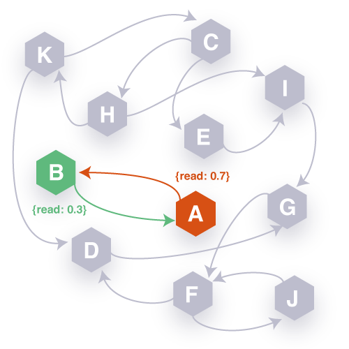
To illustrate, consider the following simplest of examples. We have a 2-node graph with nodes A and B, and edges A-to-B and B-to-A. A has the following context {read: 0.7}, while B has {read: 0.3}, that is, the likelihood that an agent in State A is reading from some data store is 0.7, and in B it is 0.3.
Imagine we have optimized our system to support high read hits. That is, we assume that most agents will be in State A and rarely transition to B. As we monitor our system, we notice that though indeed most users are in A, there is a trend towards transition to B and staying there for the duration of sessions. When do we re-evaluate our optimization model (i.e., heavily read-optimized)?
Simulations are one way to tackle this problem. We could simply generate multiple agent types that describe different types of users, by giving them different transition functions that describe how likely they are to move from one state to another, or remain put. We then vary the amount of agents in the system to see at which point we should be testing new optimizations, and at which point it is imperative that we re-optimize.
Clearly simulations may be an overkill for simple systems, but the same idea carries over to complex systems. Here we have different user types, different usage patterns, and we want to understand how sensitive our system model assumptions are to the changing user dynamics.
Running Simulations
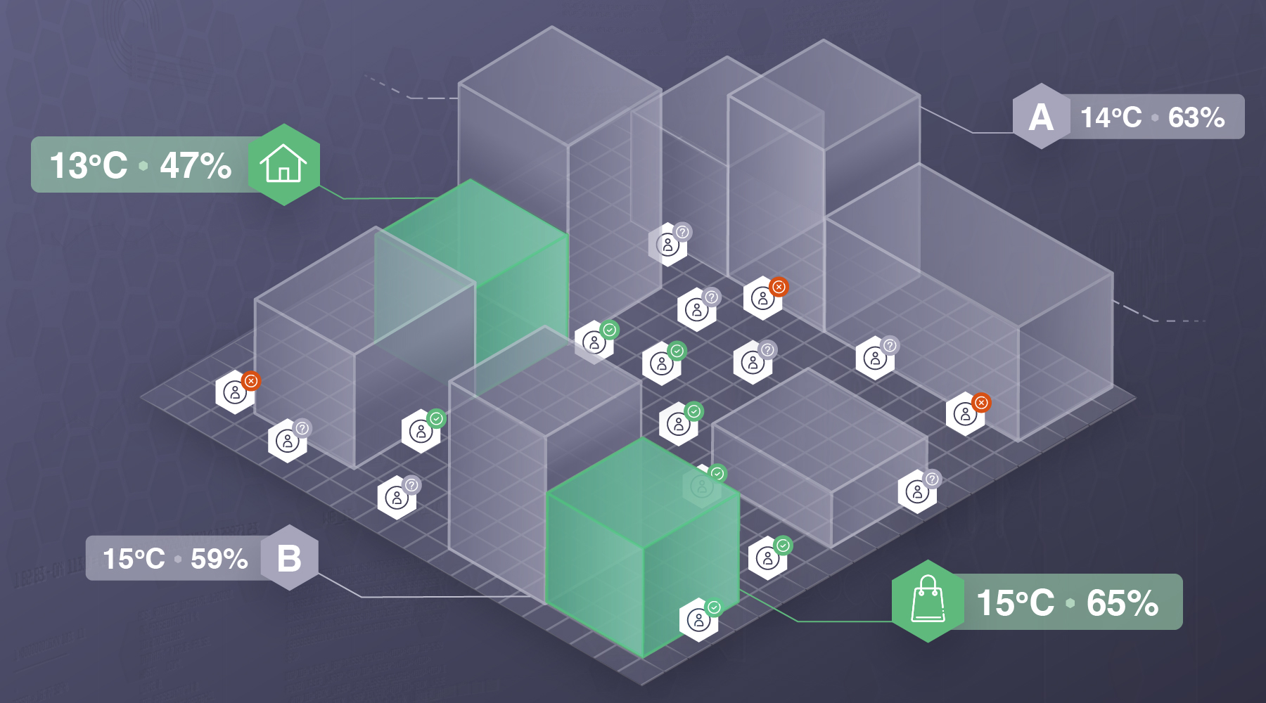
Consider a more complex case where the security decision is made based on the location context of the users. Let’s suppose that users only have a few locations as possible states, e.g. their home, their work, and their favorite coffee shop, and our system is optimized to grant access to users only when they are at home or at work (that is, their most visited places). Let’s also suppose that for this example, each location is given a set of environmental variables (e.g., ambient temperature, humidity, etc.) as context. To simulate this system, each graph node in our world is assigned a pair of temperature-humidity values. In reality, locations that are in proximity might share the same conditions, so to preserve this in our simulation, we introduce a context spread, meaning that some nodes that we define as central nodes will pass their context to their nearest neighbours.
|
|
|
|
|
|
The simulation of this system consists of two parts: the definition of a transition function for the agents and the collection of the contextual information, given the agent traces.
In real-life, people tend to spend most of their time at home or at work, while they are less likely to be found, for instance, at coffee shops. The probability that a person will go to a given location, depends on the person’s current state. This behaviour can be simulated by treating agents’ transition probabilities as Markov-chain models. Depending on how we want our agents to behave in terms of how much time they spend in each of these locations, we can define different probability distributions. As mentioned above, usually agents will spend most of their time in only a handful of locations, a behaviour that can be best represented by an exponential-like probability distribution (human agents). Even though the behaviour of the majority of agents could be effectively described by exponential transition probabilities, we might still want to consider those who exhibit more random transition patterns (random agents). That could be for instance the case for agents that are travelling; in this case, agents are allowed to randomly wander on the map for a given number of steps. As control, we can also define agents that only stay in one location at all times (stationary agents).
| Home | Work | Coffee Shop | |
|---|---|---|---|
| Home | 0.8 | 0.1 | 0.1 |
| Work | 0.15 | 0.7 | 0.15 |
| Coffee Shop | 0.6 | 0.3 | 0.1 |
Table 1: Transition probabilities for a human agent who spends most of its time at home or at work.
|
|
|
|
|
|
One way we can differentiate nodes and identify whether a particular node is e.g. the user’s home, is by looking at how frequently this place was visited. Assuming that the temperature and humidity values across the main states of a user are different, the frequency at which a certain temperature-humidity pair is encountered, corresponds to the frequency of the user being at the corresponding state. Therefore, we need to collect the contextual data that users encounter as they move in the world throughout a given period.
As we run the simulation, all agents walk in the world and visit different nodes given their transition probabilities. The path that an agent takes to transition from the origin node to the destination one, is chosen randomly from all k-shortest paths that connect the two nodes. All nodes that are visited by an agent during the simulation (along with their contextual information) are stored as the agents move. Let’s suppose that for this example, the data collection happens every 60 minutes for a period of one month. A sample of the context data that each agent collects while traversing the world is randomly retrieved at the end of the simulation.
|
|
| Agent Id | Check 1 | Check 2 | Check 3 |
|---|---|---|---|
| 1 | T: 21, H: 34, dt: Apr23-14:00 | T: 20, H: 36, dt: Apr24-17:00 | T: 14, H: 46, dt: Apr25-02:00 |
| 2 | T: 15, H: 44, dt: Apr23-14:00 | H:T: 11, H: 50, dt: Apr24-17:00 | T: 04, H: 52, dt: Apr25-02:00 |
Based on these traces, we can build a simple authentication model as follows. First, we infer the type and the behaviour of our agents, given the collected data. In particular, by looking at the frequency of each temperature-humidity pair in the collected data, we can infer the frequency at which each node was visited. In the case of human agents, some nodes will appear more times than others, whereas for the random agents all nodes will be equally present in the data. This way we can distinguish the different agent types. Second, we decide whether a particular pair is a “heavy-hitter” in the distribution. That is, we need to establish that a given pair has a high probability of uniquely representing the agent’s home or work locations.
It is beyond the scope of this article to dive into different ways of differentiating between distributions and identifying heavy-hitters, and we underline again that the generated traces ought to facilitate this selection and their training.
For the sake of simplicity, in this post we implicitly assume that temperature-humidity pairs are unique across nodes. When building real-world authentication models, we have to ensure that the entropy of the context is sufficiently high to prevent false positives.
Summary
This article shows how we define complex contextual worlds and simulate different agents in such worlds. We can then use the collected simulations (i.e. agents’ traces) to test our authentication ML models, or indeed train new models.
For example, we can use the above defined simulation, to train a model to distinguish human traces from random traces, and then make an authentication decision given a particular temperature-humidity pair (e.g. not every seen pair should be permitted). For the real-world authentication models, we would replace temperature with network and location data to build more appropriate worlds. Nevertheless, the game is still the same: define the worlds and contexts, define how we think human agents behave in such worlds, and finally collect the traces.
The source code for building our graph-based agent simulation is available in Github here.
Enjoyed the read? Why not join Futurae and help us build the world’s next generation authentication platform? We are hiring!